


You might know Richard Fichtner as a Java Champion, the person behind JCON, and XDEV’s CEO. When he shared chartjs-java-model on social media, I wanted to give it a spin. Building Chart.js configurations in Java sounded useful, especially for applications where the backend already owns the data and the rules for presenting it.
NASA’s exoplanet catalogue gives us a good reason to explore that idea further. It contains several thousand planets outside our solar system, discovered in different years and with different methods. Some have measurements we can compare; others are missing the values a particular chart. Working with this catalogue means deciding what a chart should count before choosing its colours.
We will build a Quarkus application with three connected views: discoveries by year, a breakdown of detection methods, and planet radius against orbital period. You can select a year range or click a discovery bar to inspect one year. All three views use the same selection, and the page explains why some planets appear in the counts but cannot appear on the scatter plot.
The application can read a bundled snapshot or query the live NASA archive. That gives you a repeatable demonstration and a way to explore changes in the real data. Along the way, we will keep the data rules in Java, build chart configurations with XDEV’s model, and give the browser responsibility for rendering and interaction.
Choose the question before the chart
The NASA Exoplanet Archive’s TAP service accepts a SQL-like query and can return JSON without an API key. TAP stands for Table Access Protocol. We use its synchronous endpoint: send a query, wait for the response, and deserialize the returned rows. The projection we need is small enough to fetch as one catalogue.
There is a counting problem in the data though. The Planetary Systems table, ps, can contain several published parameter sets for the same planet. Counting its rows would count some planets more than once. We select default_flag=1 to obtain the archive’s default parameter set for each planet, then validate that the resulting names are unique. NASA documents all fields in its table definitions.
The alternative composite table fills more gaps by combining references and sometimes calculating values. For this example, we use the default solutions from ps and make their missing measurements visible. The choice becomes part of our application contract: every discovery counts once, even when the selected solution lacks a radius.
These are the questions the dashboard will answer:
Discoveries by year: The stacked bars show how many planets in the catalogue have each discovery year. Java counts each planet once and includes years with zero discoveries.
Discovery methods: The doughnut chart shows which methods discovered those planets. Java applies the same year filter and keeps the method groups consistent.
Planet comparisons: The scatter plot shows the available sizes and orbital periods. Java selects suitable measurement pairs and reports how many planets were excluded from this view.
The snapshot I downloaded when building this tutorial contains 6,360 unique planets. Its default 1992–2025 selection contains 6,089, of which 4,513 have usable period and radius values. The other 1,576 remain in the discovery counts.
These charts describe the catalogue. They do not tell us how common each kind of planet is across the universe. Different detection methods favour different observable properties. The current year is also incomplete, which is why the initial range ends in 2025.
Put the responsibilities in the right place
If you have built a REST application before, most of this design will look familiar. A client reads an external service, an application service keeps a reusable representation, and a resource returns a response. The new part is the chart configuration: it becomes another Java object assembled from the selected data.
The data flows through the application like this:
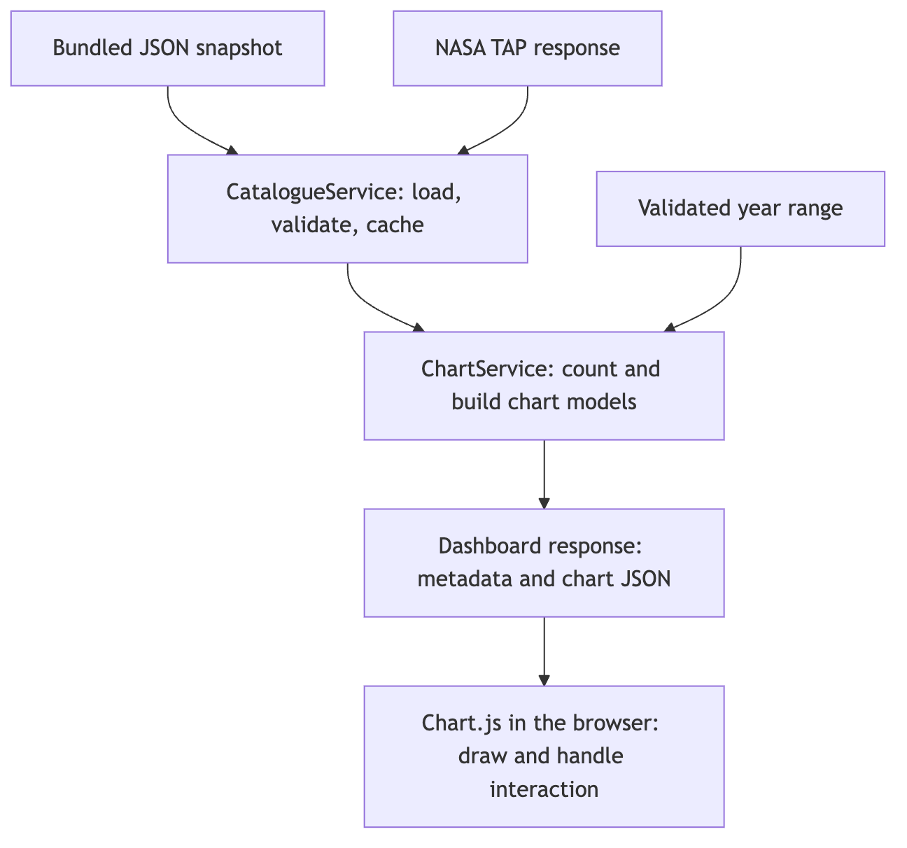
The catalogue is shared between requests. The chart configurations are built afresh for each range. This distinction is important because the chart models use mutable setters, while a cached catalogue should not change underneath another request.
There is also a boundary between a chart description and executable browser behaviour. XDEV’s library supplies Java models for Chart.js configurations; it does not draw the charts on the server. Chart.js still needs to run in the browser, and JavaScript callbacks still belong there. We will cross that boundary through JSON and attach the callbacks after the response arrives.
Create the application
You need JDK 25, the Quarkus CLI, Python 3, curl, and a current browser. The commands below use a POSIX shell, such as Bash or Zsh. The generated Maven wrapper handles the build, and Python’s standard library handles the snapshot download.
Initial dependency, data, and browser-library downloads require internet access. Once those are present, the snapshot path runs locally. No database, account, container, or frontend build tool is needed for this application.
But now let’s get started. Run the following command from the directory where you keep demo projects or start from my Github repository:
quarkus create app com.themainthread:quarkus-exoplanet-charts \
  -P io.quarkus.platform:quarkus-bom:3.39.1 \
  --java=25 --no-dockerfiles \
  --extensions=rest-jackson,rest-client-jackson,cache
cd quarkus-exoplanet-charts
Quarkus REST serves our JSON endpoint. The REST client reads NASA’s response, and the cache keeps range changes from downloading the catalogue again. The CLI creates the Maven configuration, including the test dependencies and the plugins needed to test the packaged application. Keep those generated settings.
Remove the generated greeting endpoint and its two tests; we will create the dashboard and its tests as part of the article:
rm src/main/java/com/themainthread/GreetingResource.java \
  src/test/java/com/themainthread/GreetingResourceTest.java \
  src/test/java/com/themainthread/GreetingResourceIT.java
The platform manages the Quarkus dependencies. The chart library is outside that dependency management, so add it inside pom.xml‘s existing <dependencies> element:
<dependency>
    <groupId>software.xdev</groupId>
    <artifactId>chartjs-java-model</artifactId>
    <version>3.0.2</version>
</dependency>
Version 3 moved the library to Jackson 3. Its release source supplies a configured writer through toJson(), while our Quarkus REST extension uses Jackson 2. We will let the library serialize its chart models, then parse that JSON into the tree representation used by our REST response. This keeps the library’s serialization rules in effect without replacing Quarkus’s mapper.
Create the directories for the remaining files:
mkdir -p src/main/java/com/themainthread/exoplanets \
  src/test/java/com/themainthread/exoplanets \
  src/main/resources/data \
  src/main/resources/META-INF/resources/vendor \
  scripts
Download a catalogue you can reproduce
We need seven columns: a name, a discovery method, a discovery year, and two measurements with their limit flags. Create src/main/resources/data/query.sql:
select pl_name,discoverymethod,disc_year,pl_orbper,pl_orbperlim,pl_rade,pl_radelim from ps where default_flag=1 order by pl_nameThe column definitions give the units: orbital period is in days, and radius is in Earth radii. The associated lim columns distinguish measurements from limits. The discovery year describes the discovery.
The query deliberately leaves out the year range and measurement filters. We need the full selected catalogue to support range changes, and we need incomplete rows to count discoveries correctly. Keeping the query in a file also gives the live client and the snapshot downloader the same projection. Browser input will never be concatenated into this SQL.
Create scripts/refresh-snapshot.py:
#!/usr/bin/env python3
"""Download the exact TAP projection used by the application. Requires Python 3."""

import hashlib
import json
from datetime import datetime, timezone
from pathlib import Path
from urllib.parse import urlencode
from urllib.request import Request, urlopen

ROOT = Path(__file__).resolve().parents[1]
DATA = ROOT / "src/main/resources/data"
query = (DATA / "query.sql").read_text().strip()
url = "https://exoplanetarchive.ipac.caltech.edu/TAP/sync?" + urlencode({"query": query, "format": "json"})
request = Request(url, headers={"Accept": "application/json", "User-Agent": "TheMainThread-ExoplanetTutorial/1.0"})
with urlopen(request, timeout=60) as response:
    planets = json.load(response)
fields = {"pl_name", "discoverymethod", "disc_year", "pl_orbper", "pl_orbperlim", "pl_rade", "pl_radelim"}
if not isinstance(planets, list) or not planets:
    raise SystemExit("Expected a non-empty JSON array; the existing snapshot is unchanged.")
if any(not isinstance(row, dict) or not fields.issubset(row) for row in planets):
    raise SystemExit("The archive response is missing required fields; the existing snapshot is unchanged.")
names = [row["pl_name"] for row in planets]
if any(not isinstance(name, str) or not name.strip() for name in names) or len(set(names)) != len(names):
    raise SystemExit("Expected one named row per planet; the existing snapshot is unchanged.")
snapshot = {"retrievedAt": datetime.now(timezone.utc).isoformat().replace("+00:00", "Z"),
            "query": query, "planets": planets}
target = DATA / "snapshot.json"
temporary = target.with_suffix(".json.tmp")
temporary.write_text(json.dumps(snapshot, indent=2, ensure_ascii=False) + "\n")
temporary.replace(target)
print(f"Saved {len(planets)} planets to {target}")
print(f"Retrieved: {snapshot['retrievedAt']}")
print(f"SHA-256: {hashlib.sha256(target.read_bytes()).hexdigest()}")
The script requests JSON and checks its structure before replacing the previous snapshot. It rejects an empty response, missing columns, blank names, and duplicate names. It then wraps the rows with the exact query and a retrieval timestamp. Writing to a temporary file first means the previous snapshot remains available if the request or validation fails.
Run it from the module directory:
python3 scripts/refresh-snapshot.pyYou should get a non-empty src/main/resources/data/snapshot.json and three output lines containing the record count, retrieval time, and SHA-256.
Before writing Java, inspect the downloaded result:
python3 - <<'PY_SNAPSHOT'
import json
from pathlib import Path
snapshot = json.loads(Path('src/main/resources/data/snapshot.json').read_text())
planets = snapshot['planets']
assert planets and len({p['pl_name'] for p in planets}) == len(planets)
years = [p['disc_year'] for p in planets if p['disc_year'] is not None]
print('Retrieved:', snapshot['retrievedAt'])
print('Planets:', len(planets))
print('Discovery years:', min(years), 'to', max(years))
PY_SNAPSHOT
The snapshot for me reported 6,360 planets and discovery years from 1992 to 2026. If you are following the listings in a new project, the downloader creates your own snapshot.
Preserve missing values in Java
Now we can give the archive response a Java representation. Create src/main/java/com/themainthread/exoplanets/Planet.java:
package com.themainthread.exoplanets;

import com.fasterxml.jackson.annotation.JsonProperty;

public record Planet(
        @JsonProperty("pl_name") String name,
        @JsonProperty("discoverymethod") String method,
        @JsonProperty("disc_year") Integer year,
        @JsonProperty("pl_orbper") Double period,
        @JsonProperty("pl_orbperlim") Integer periodLimit,
        @JsonProperty("pl_rade") Double radius,
        @JsonProperty("pl_radelim") Integer radiusLimit) {

    public boolean hasMeasuredSizeAndPeriod() {
        return positive(period) && positive(radius)
                && Integer.valueOf(0).equals(periodLimit)
                && Integer.valueOf(0).equals(radiusLimit);
    }

    private static boolean positive(Double value) {
        return value != null && Double.isFinite(value) && value > 0;
    }
}
The wrapper types are necessary. A missing radius can remain null, which lets the application distinguish it from a numeric value. The JSON annotations keep the archive’s column names at the client boundary while giving the rest of the Java code shorter names such as period() and radius().
The predicate answers a specific question: can this row supply a point for our period-and-radius comparison? Both values must be finite and positive, and both limit flags must be zero.
The positive-value check serves the logarithmic axes we will use later. Values of zero or less cannot be placed on those axes.
“Measured” here means that the selected values meet these conditions. It does not establish scientific quality, and this dashboard does not draw uncertainty intervals. Exclusion also does not mean that no radius has ever been published for a planet. It means the default parameter set selected by our query does not supply the pair we need.
Create Catalogue.java in the same package:
package com.themainthread.exoplanets;

import java.util.List;

public record Catalogue(String retrievedAt, String query, List<Planet> planets) {
    public Catalogue {
        planets = List.copyOf(planets);
    }
}
List.copyOf() prevents a caller from adding or removing rows in a shared catalogue. The rows themselves are records containing immutable values. We can therefore cache this representation and let concurrent requests read it, while keeping each request’s mutable chart builders separate.
Load the snapshot or call NASA
The live path needs one REST client method. Create ArchiveClient.java in the same package:
package com.themainthread.exoplanets;

import java.util.List;

import jakarta.ws.rs.GET;
import jakarta.ws.rs.Path;
import jakarta.ws.rs.Produces;
import jakarta.ws.rs.QueryParam;
import jakarta.ws.rs.core.MediaType;

import org.eclipse.microprofile.rest.client.inject.RegisterRestClient;

@Path("/TAP/sync")
@RegisterRestClient(configKey = "nasa")
public interface ArchiveClient {
    @GET
    @Produces(MediaType.APPLICATION_JSON)
    List<Planet> query(@QueryParam("query") String query, @QueryParam("format") String format);
}
@RegisterRestClient(configKey = "nasa") connects the interface to a configured base URL. The client adds /TAP/sync, encodes the query parameters, and deserializes the response into List<Planet>. That encoding matters here because the SQL contains spaces and an equals sign. Passing the query through @QueryParam keeps those details out of the application service.
Add these settings to src/main/resources/application.properties:
quarkus.rest-client.nasa.url=https://exoplanetarchive.ipac.caltech.edu
quarkus.rest-client.nasa.connect-timeout=5000
quarkus.rest-client.nasa.read-timeout=60000
quarkus.cache.caffeine.catalogue.maximum-size=2
quarkus.cache.caffeine.catalogue.expire-after-write=1h
The REST client timeouts are in milliseconds. We allow up to five seconds to establish a connection and up to a minute for a response read. Those settings bound separate stages of the client call; they are not a promise that every dashboard request completes within exactly one minute.
The catalogue cache has room for two entries because this application has two source choices, snapshot and live. Each entry expires an hour after it is written. We apply the cache to loading a catalogue, so selecting a different year range will not create another cached copy of the same NASA response.
Create CatalogueService.java:
package com.themainthread.exoplanets;

import java.io.IOException;
import java.io.InputStream;
import java.nio.charset.StandardCharsets;
import java.time.Instant;
import java.util.HashSet;

import jakarta.enterprise.context.ApplicationScoped;

import org.eclipse.microprofile.rest.client.inject.RestClient;

import com.fasterxml.jackson.databind.ObjectMapper;

import io.quarkus.cache.CacheResult;

@ApplicationScoped
public class CatalogueService {
    public enum Source { snapshot, live }

    private final ArchiveClient client;
    private final ObjectMapper mapper;

    public CatalogueService(@RestClient ArchiveClient client, ObjectMapper mapper) {
        this.client = client;
        this.mapper = mapper;
    }

    @CacheResult(cacheName = "catalogue")
    public Catalogue load(Source source) {
        try {
            Catalogue catalogue;
            if (source == Source.snapshot) {
                try (InputStream input = resource("snapshot.json")) {
                    catalogue = mapper.readValue(input, Catalogue.class);
                }
            } else {
                String query;
                try (InputStream input = resource("query.sql")) {
                    query = new String(input.readAllBytes(), StandardCharsets.UTF_8).strip();
                }
                var planets = client.query(query, "json");
                catalogue = new Catalogue(Instant.now().toString(), query, planets);
            }
            validate(catalogue);
            return catalogue;
        } catch (IOException | RuntimeException exception) {
            throw new CatalogueUnavailableException("Could not load the " + source + " catalogue", exception);
        }
    }

    private static InputStream resource(String name) throws IOException {
        InputStream input = CatalogueService.class.getResourceAsStream("/data/" + name);
        if (input == null) {
            throw new IOException("Missing data/" + name);
        }
        return input;
    }

    private static void validate(Catalogue catalogue) {
        if (catalogue.planets().isEmpty()) {
            throw new IllegalArgumentException("Archive returned an empty catalogue");
        }
        var names = new HashSet<String>();
        for (Planet planet : catalogue.planets()) {
            if (planet.name() == null || planet.name().isBlank() || !names.add(planet.name())) {
                throw new IllegalArgumentException("Expected one named row per planet");
            }
        }
    }

    public static class CatalogueUnavailableException extends RuntimeException {
        public CatalogueUnavailableException(String message, Throwable cause) {
            super(message, cause);
        }
    }
}
Both branches return the same Catalogue type. The snapshot branch reads the wrapper document created by Python. The live branch reads the query resource, calls the REST client, and attaches a timestamp after the response arrives. The resource helper uses classpath streams so the same code works when the files are packaged inside the application. Validation happens before the result is returned and cached.
@CacheResult is applied to a CDI bean method. The resource will call that bean through injection, allowing Quarkus to intercept the call and reuse the result. Since source is its only argument, that argument identifies the cache entry. The Quarkus cache guide describes this key selection and the cache lifecycle.
If the live request fails, the resource will return an error. The user can then choose the snapshot explicitly. That choice keeps the source and retrieval date accurate: the application never labels an old bundled file as a successful live response.
Work through the counting rules
Before looking at the chart API, it helps to follow a small selection by hand. The following planets are synthetic test fixtures, not astronomical observations. Assume the selected range is 2000–2002 and that the valid measurement pairs have zero limit flags:
Planet A was discovered by Transit in 2000. Its period is 4 days and its radius is 2 Earth radii, so it contributes one discovery and one scatter point.
Planet B was discovered by Radial Velocity in 2002. Its radius is missing, so it contributes one discovery but no scatter point.
Planet C was discovered by Imaging in 2002. Its period is a limit, so it also contributes one discovery but no scatter point.
Planet D was discovered by an unfamiliar method, New technique, in 2002. Its period is 20 days and its radius is 1.5 Earth radii, so it contributes one discovery and one scatter point, both in the Other group.
Planet E was discovered by Transit and has a valid measurement pair, but its discovery year is missing. It contributes neither a selected discovery nor a scatter point.
Planet F was discovered by Transit in 2020 and has a valid measurement pair. It falls outside the selected range, so it contributes neither a selected discovery nor a scatter point.
Four planets belong to the range, and two of them can be plotted. Planet E cannot be assigned to a year, so it contributes to an unknownYear count for the catalogue. Planet F is outside the requested range. Neither belongs in the four selected discoveries.
The bar labels must still contain 2000, 2001, and 2002. Their totals are 1, 0, and 3. If each method built labels from only its own discoveries, the arrays could disagree about what their second position means. We avoid that ambiguity by allocating every year position first and incrementing the corresponding count.
The doughnut chart uses totals from those same arrays. The scatter plot uses the eligible rows retained during the same pass. That gives us a useful invariant for every response: selected = plotted + excludedFromScatter. It also explains why a planet with missing measurements remains visible in the two discovery views.
Build the chart configurations in Java
Create ChartService.java in src/main/java/com/themainthread/exoplanets:
package com.themainthread.exoplanets;

import java.io.IOException;
import java.util.ArrayList;
import java.util.List;

import jakarta.enterprise.context.ApplicationScoped;

import com.fasterxml.jackson.databind.JsonNode;
import com.fasterxml.jackson.databind.ObjectMapper;
import com.fasterxml.jackson.databind.node.ObjectNode;

import software.xdev.chartjs.model.charts.BarChart;
import software.xdev.chartjs.model.charts.Chart;
import software.xdev.chartjs.model.charts.DoughnutChart;
import software.xdev.chartjs.model.charts.ScatterChart;
import software.xdev.chartjs.model.data.BarData;
import software.xdev.chartjs.model.data.DoughnutData;
import software.xdev.chartjs.model.data.ScatterData;
import software.xdev.chartjs.model.datapoint.ScatterDataPoint;
import software.xdev.chartjs.model.dataset.BarDataset;
import software.xdev.chartjs.model.dataset.DoughnutDataset;
import software.xdev.chartjs.model.dataset.ScatterDataset;
import software.xdev.chartjs.model.options.BarOptions;
import software.xdev.chartjs.model.options.DoughnutOptions;
import software.xdev.chartjs.model.options.LineOptions;
import software.xdev.chartjs.model.options.scale.Scales;
import software.xdev.chartjs.model.options.scale.cartesian.AbstractCartesianScaleOptions.Title;
import software.xdev.chartjs.model.options.scale.cartesian.category.CategoryScaleOptions;
import software.xdev.chartjs.model.options.scale.cartesian.linear.LinearScaleOptions;
import software.xdev.chartjs.model.options.scale.cartesian.logarithmic.LogarithmicScaleOptions;

@ApplicationScoped
public class ChartService {
    private static final List<String> METHODS = List.of("Transit", "Radial Velocity", "Microlensing", "Imaging", "Other");
    private static final List<String> COLORS = List.of("#5eead4", "#fbbf24", "#a78bfa", "#fb7185", "#94a3b8");
    private final ObjectMapper mapper;

    public ChartService(ObjectMapper mapper) {
        this.mapper = mapper;
    }

    public Dashboard build(Catalogue catalogue, String source, int from, int to) {
        int[][] counts = new int[METHODS.size()][to - from + 1];
        List<List<Planet>> measured = new ArrayList<>();
        for (String ignored : METHODS) {
            measured.add(new ArrayList<>());
        }
        int selected = 0;
        int unknownYear = 0;
        for (Planet planet : catalogue.planets()) {
            if (planet.year() == null) {
                unknownYear++;
                continue;
            }
            if (planet.year() < from || planet.year() > to) {
                continue;
            }
            selected++;
            int group = planet.method() == null ? -1 : METHODS.indexOf(planet.method());
            if (group < 0) {
                group = METHODS.size() - 1;
            }
            counts[group][planet.year() - from]++;
            if (planet.hasMeasuredSizeAndPeriod()) {
                measured.get(group).add(planet);
            }
        }

        var annual = new BarData();
        for (int year = from; year <= to; year++) {
            annual.addLabel(Integer.toString(year));
        }
        var methods = new DoughnutData();
        var methodDataset = new DoughnutDataset().setLabel("Planets");
        var scatter = new ScatterData();
        int plotted = 0;
        for (int group = 0; group < METHODS.size(); group++) {
            String label = METHODS.get(group);
            String color = COLORS.get(group);
            var yearlyDataset = new BarDataset().setLabel(label).setBackgroundColor(color);
            int total = 0;
            for (int count : counts[group]) {
                yearlyDataset.addData(count);
                total += count;
            }
            annual.addDataset(yearlyDataset);
            methods.addLabel(label);
            methodDataset.addData(total).addBackgroundColor(color);

            var points = new ScatterDataset().setLabel(label).setBackgroundColor(color)
                    .setShowLine(false).setPointRadius(List.of(3));
            for (Planet planet : measured.get(group)) {
                points.addData(new NamedPoint(planet));
                plotted++;
            }
            scatter.addDataset(points);
        }
        methods.addDataset(methodDataset);

        var annualOptions = new BarOptions().setResponsive(true).setMaintainAspectRatio(false).setAnimation(false)
                .setScales(new Scales()
                        .addScale("x", new CategoryScaleOptions().setStacked(true).setTitle(title("Discovery year")))
                        .addScale("y", new LinearScaleOptions().setStacked(true).setBeginAtZero(true)
                                .setTitle(title("Planets"))));
        var scatterOptions = new LineOptions().setResponsive(true).setMaintainAspectRatio(false).setAnimation(false)
                .setScales(new Scales()
                        .addScale("x", new LogarithmicScaleOptions().setTitle(title("Orbital period (days, log scale)")))
                        .addScale("y", new LogarithmicScaleOptions().setTitle(title("Radius (Earth radii, log scale)"))));
        var methodOptions = new DoughnutOptions().setResponsive(true).setMaintainAspectRatio(false).setAnimation(false);

        return new Dashboard(source, catalogue.retrievedAt(), from, to, catalogue.planets().size(),
                selected, plotted, selected - plotted, unknownYear,
                json(new BarChart(annual, annualOptions)),
                json(new DoughnutChart(methods, methodOptions)),
                json(new ScatterChart(scatter, scatterOptions)));
    }

    private JsonNode json(Chart<?, ?, ?> chart) {
        try {
            // Preserve the library's Jackson 3 serializers, then embed an object in our Jackson response.
            JsonNode node = mapper.readTree(chart.toJson());
            // The library omits empty collections. Chart.js expects each dataset to have a data array.
            for (JsonNode dataset : node.path("data").path("datasets")) {
                if (!dataset.has("data")) {
                    ((ObjectNode) dataset).putArray("data");
                }
            }
            return node;
        } catch (IOException exception) {
            throw new IllegalStateException("Chart serialization did not produce JSON", exception);
        }
    }

    private static Title title(String text) {
        return new Title().setDisplay(true).setText(text);
    }

    public static class NamedPoint extends ScatterDataPoint {
        private final String name;

        public NamedPoint(Planet planet) {
            super(planet.period(), planet.radius());
            name = planet.name();
        }
    }

    public record Dashboard(String source, String retrievedAt, int from, int to, int catalogueTotal,
            int selected, int plotted, int excludedFromScatter, int unknownYear,
            JsonNode discoveries, JsonNode methods, JsonNode sizes) {
    }
}
The first part of build() implements the selection we just worked through. The outer dimension of counts represents method groups, and the inner dimension represents years. Subtracting from from a discovery year gives its array position. Once a planet is inside the range, its discovery is counted before we ask whether its measurements can be plotted.
There are four named groups: Transit, Radial Velocity, Microlensing, and Imaging. Every other method, including a missing method, joins Other. This is a display choice made by the application. Keeping the labels and colours in fixed lists gives each group the same position and appearance in all three charts, including ranges where a group has no discoveries.
Match datasets to the question
The bar chart receives one dataset per method. Each dataset contains one number for every label, including zero-count years. Setting stacked on both axes lets the contributions for a year form one bar whose total is the number of discoveries. The vertical axis starts at zero because the bar length represents a count.
The doughnut chart has a different shape: one dataset holds the total for every method label. Those totals come from the bar counts, so there is no second filtering rule to keep in sync. If you add a method group later, the arrays, labels, and colours must all continue to agree on its index.
The scatter chart receives one dataset per method, with an x and y value for each eligible planet. We use orbital period for x and radius for y. setShowLine(false) leaves the observations as individual points; there is no ordering that would make a connecting line meaningful in this comparison.
NamedPoint extends the model’s ScatterDataPoint with a planet name. The library’s configured writer includes that field alongside the coordinates. The browser can then show the name and values in a tooltip without searching a separate list or making another request.
Let the scales position the original measurements
Periods and radii span a wide range, so both scatter axes are logarithmic. Equal distances on a logarithmic axis represent equal ratios. A period of 10 days sits between 1 and 100 days in logarithmic space, while the tooltip can still show its original value of 10.
We send the original positive values and configure LogarithmicScaleOptions for the axes. Applying Math.log10() in Java as well would transform the data twice and change the meaning of the tooltip values. Keeping units in the axis titles and callbacks makes the relationship explicit for the reader of the dashboard.
The options also disable animation and aspect-ratio preservation. Animation is unnecessary for the comparisons we make here, and the page will give each chart an explicit container height. Those settings are presentation choices; they do not alter the selected data.
Cross the JSON boundary deliberately
The json() method is small, but it carries an important integration decision. chart.toJson() uses the library’s Jackson 3 writer and its serialization configuration. Quarkus’s ObjectMapper then reads the resulting text into a JsonNode, which can be embedded as an object in the dashboard response.
If Dashboard stored that text in a String field, the HTTP serializer would correctly encode it as a JSON string. The browser would receive quoted chart JSON and would need another parse step before accessing data or options. Using JsonNode means response.json() yields the complete dashboard object in one step. We pay for a serialization and parse operation per chart to keep this boundary explicit.
The adapter also repairs empty dataset arrays. The model library’s writer omits empty collections, so a method with no scatter points can lose its data property. Adding data: [] gives both Chart.js and our table renderer a consistent shape. This is why an empty selection deserves a test: a well-populated catalogue can conceal a missing property that appears only when you narrow the range.
The Java model covers the chart types and options used here. Its project notes incomplete API coverage, so compile-time checks do not establish that every Chart.js feature is represented.
Expose one dashboard response
Create DashboardResource.java in the same package:
package com.themainthread.exoplanets;

import java.time.Year;
import java.util.Map;

import jakarta.ws.rs.DefaultValue;
import jakarta.ws.rs.GET;
import jakarta.ws.rs.Path;
import jakarta.ws.rs.Produces;
import jakarta.ws.rs.QueryParam;
import jakarta.ws.rs.core.MediaType;
import jakarta.ws.rs.core.Response;

import org.jboss.logging.Logger;

import com.themainthread.exoplanets.CatalogueService.CatalogueUnavailableException;
import com.themainthread.exoplanets.CatalogueService.Source;

@Path("/api/dashboard")
@Produces(MediaType.APPLICATION_JSON)
public class DashboardResource {
    private static final Logger LOG = Logger.getLogger(DashboardResource.class);
    private final CatalogueService catalogues;
    private final ChartService charts;

    public DashboardResource(CatalogueService catalogues, ChartService charts) {
        this.catalogues = catalogues;
        this.charts = charts;
    }

    @GET
    public Response dashboard(@QueryParam("source") @DefaultValue("snapshot") String source,
            @QueryParam("from") @DefaultValue("1992") String fromText,
            @QueryParam("to") @DefaultValue("2025") String toText) {
        int from;
        int to;
        Source selectedSource;
        try {
            from = Integer.parseInt(fromText);
            to = Integer.parseInt(toText);
            selectedSource = Source.valueOf(source);
        } catch (IllegalArgumentException exception) {
            return error(400, "Use integer years and source=snapshot or source=live.");
        }
        if (from < 1992 || to > Year.now().getValue() || from > to) {
            return error(400, "Years must be ordered and between 1992 and the current year.");
        }
        try {
            return Response.ok(charts.build(catalogues.load(selectedSource), source, from, to))
                    .header("Cache-Control", "no-store").build();
        } catch (CatalogueUnavailableException exception) {
            LOG.warn("Catalogue request failed", exception);
            return error(503, "Catalogue unavailable. Retry later or choose the bundled snapshot.");
        }
    }

    private static Response error(int status, String message) {
        return Response.status(status).entity(Map.of("error", message)).header("Cache-Control", "no-store").build();
    }
}
The endpoint receives its query parameters as strings so it can return the same JSON error shape for malformed numbers and unknown sources. It then checks the year ordering and bounds before calling either service. The lower bound is 1992, and the upper bound is the current year. The default upper year stays fixed at 2025 to keep the initial view on completed years.
One response contains all three chart configurations from one loaded catalogue and one validated range. It also carries the source, retrieval time, total catalogue size, selected count, plotted count, scatter exclusions, and missing-year count. A missing discovery year is reported across the loaded catalogue because it cannot be assigned to the requested interval.
Invalid input returns HTTP 400. A catalogue loading failure returns HTTP 503 with a message the page can display, while the underlying exception is logged on the server. A valid year range with no discoveries is different: it returns HTTP 200 with zero counts and empty chart datasets.
The method returns a synchronous Response, so Quarkus REST runs this blocking work on a worker thread. Cache-Control: no-store applies to the HTTP response. It does not disable the server’s catalogue cache; the browser requests a dashboard response while Quarkus can reuse the loaded data behind it.
Start the application from the module directory:
./mvnw quarkus:devWait for Quarkus to report that it is listening on port 8080. In another terminal, check the endpoint before adding the page:
curl -fsS 'http://localhost:8080/api/dashboard?from=1992&to=2025' \
  -o /tmp/exoplanet-dashboard.json
python3 - <<'PY_CHECK'
import json
with open('/tmp/exoplanet-dashboard.json') as source:
    data = json.load(source)
assert data['selected'] == data['plotted'] + data['excludedFromScatter']
assert data['discoveries']['type'] == 'bar'
assert data['methods']['type'] == 'doughnut'
assert data['sizes']['options']['scales']['x']['type'] == 'logarithmic'
assert sum(data['methods']['data']['datasets'][0]['data']) == data['selected']
print(data['source'], data['selected'], data['plotted'], data['excludedFromScatter'])
PY_CHECK
With the supplied snapshot, the last line is snapshot 6089 4513 1576. A freshly downloaded snapshot can differ. The assertions check relationships that should remain true across catalogue updates, including that the method totals account for every selected planet.
If this request fails, resolve it before adding browser code. Check that the snapshot exists under src/main/resources/data and that the application has started successfully. A working JSON endpoint gives us a known starting point for the rendering step.
Bundle Chart.js with Quarkus
The Java model library describes the charts. The browser still needs Chart.js to render them. Quarkus Web Bundler brings that renderer into the Maven build and bundles it with our JavaScript and CSS.
Stop dev mode with Ctrl+C, then add the extension from the module directory:
quarkus extension add io.quarkiverse.web-bundler:quarkus-web-bundler:2.3.4Web Bundler accepts browser libraries as Maven dependencies through mvnpm. Add the pinned Chart.js dependency to the existing <dependencies> element in pom.xml:
<dependency>
    <groupId>org.mvnpm</groupId>
    <artifactId>chart.js</artifactId>
    <version>4.5.1</version>
    <scope>provided</scope>
</dependency>
The provided scope makes Chart.js available to the build without shipping its dependency JAR in the running application. The generated JavaScript contains the browser code we import. This is independent of software.xdev:chartjs-java-model, which remains a Java dependency used by ChartService.
Add node_modules/ to the generated .gitignore. Web Bundler creates this directory from the Maven dependencies; you do not run npm install or maintain a separate package.json for this example.
Keep the renderer’s license with the application as well:
curl -fsSL https://cdn.jsdelivr.net/npm/chart.js@4.5.1/LICENSE.md \
  -o src/main/resources/web/public/vendor/Chart.js-LICENSE.md
Files under web/public are served unchanged. The application scripts and styles belong directly under src/main/resources/web, where Web Bundler discovers them for the default app bundle.
Create src/main/resources/META-INF/resources/index.html:
<!doctype html>
<html lang="en">
<head>
    <meta charset="utf-8">
    <meta name="viewport" content="width=device-width,initial-scale=1">
    <title>Worlds beyond our own · The Main Thread</title>
    <link rel="stylesheet" href="/style.css">
    <script defer src="/vendor/chart.umd.min.js"></script>
    <script defer src="/app.js"></script>
</head>
<body>
<main>
    <header>
        <p class="eyebrow">THE MAIN THREAD <span>/</span> EXOPLANET EXPLORER</p>
        <h1>Worlds beyond<br><em>our own.</em></h1>
        <p class="intro">Explore the planets we have found, how we found them, and the measurements we have. One catalogue. Three views.</p>
    </header>
    <form id="filters">
        <label>Catalogue<select name="source"><option value="snapshot">Bundled snapshot</option><option value="live">NASA archive · live</option></select></label>
        <label>From year<input name="from" type="number" min="1992" value="1992" required></label>
        <label>To year<input name="to" type="number" min="1992" value="2025" required></label>
        <button type="submit">Explore range <span aria-hidden="true">↗</span></button>
        <button id="reset" type="button" class="secondary">Reset years</button>
    </form>
    <p id="status" role="status" aria-live="polite">Loading the catalogue…</p>
    <section id="results" hidden>
        <div class="metrics">
            <div><span id="selected">—</span><p>planets in this range</p></div>
            <div><span id="plotted">—</span><p>with usable size + period</p></div>
            <div><span id="excluded">—</span><p>excluded from the scatter plot</p></div>
        </div>
        <div class="chart-grid">
            <section class="panel annual">
                <p class="eyebrow">01 / DISCOVERY</p><h2>How the catalogue grew</h2>
                <p>Planets by discovery year, grouped by detection method. Click a bar to explore that year.</p>
                <div class="canvas-wrap"><canvas id="discoveries" role="img" aria-label="Stacked chart of planets by discovery year and method. Values are available in the table below."></canvas></div>
            </section>
            <section class="panel">
                <p class="eyebrow">02 / DETECTION</p><h2>How we found them</h2>
                <p>Discovery methods in the selected range. Smaller method categories are grouped as Other.</p>
                <div class="canvas-wrap"><canvas id="methods" role="img" aria-label="Doughnut chart of discovery methods. Values are available in the table below."></canvas></div>
            </section>
            <section class="panel scatter">
                <p class="eyebrow">03 / COMPARISON</p><h2>A year on another world</h2>
                <p>Orbital period versus planet radius. Each dot is one planet. Both axes use a logarithmic scale; hover for its name and values.</p>
                <div class="canvas-wrap tall"><canvas id="sizes" role="img" aria-label="Scatter plot of orbital period in days and radius in Earth radii. Point values are available in the table below."></canvas></div>
                <p class="note">Only finite, positive values with both limit flags equal to zero are plotted. Missing measurements and upper or lower limits are excluded. Measurement uncertainties are not shown.</p>
            </section>
        </div>
        <details><summary>Read the chart values as tables</summary><div id="tables"></div></details>
        <aside><h2>A catalogue of discoveries</h2><p>These charts describe known planets and the measurements available for them. Detection methods favour different kinds of planets, so the plots do not estimate how common each kind is in the universe. The current year is incomplete; the default range ends in 2025.</p></aside>
        <p id="provenance" class="note"></p>
    </section>
    <footer>Data: <a href="https://exoplanetarchive.ipac.caltech.edu/">NASA Exoplanet Archive</a> · <a href="https://exoplanetarchive.ipac.caltech.edu/docs/acknowledge.html">Attribution</a><br>Built with Quarkus, <a href="https://github.com/xdev-software/chartjs-java-model">chartjs-java-model</a>, and Chart.js.</footer>
</main>
</body>
</html>
The form owns the source and year range, and the three canvases have stable IDs matching the chart fields in the response. Both scripts use defer, with Chart.js listed first, so the library and page elements are available when app.js starts. The status element reports loading, selection, and error messages outside the initially hidden results section.
Create style.css alongside index.html.
:root { color-scheme: dark; font-family: system-ui, sans-serif; color: #e5edf5; background: #080e18; }
* { box-sizing: border-box; }
body { margin: 0; background: radial-gradient(ellipse at 92% 0%, #17303d 0, transparent 40%); }
main { max-width: 1360px; padding: 52px 48px 30px; margin: auto; }
header { padding-bottom: 34px; }
.eyebrow { font: 11px ui-monospace, monospace; letter-spacing: .15em; color: #9bafc4; }
.eyebrow span { margin: 0 12px; color: #5eead4; }
h1 { font-size: clamp(44px, 5.8vw, 78px); line-height: 1.04; font-weight: 570; letter-spacing: -.06em; margin: 26px 0 20px; }
h1 em { color: #5eead4; font-family: Georgia, serif; font-weight: 400; }
.intro { max-width: 610px; font-size: 17px; line-height: 1.6; color: #a8bacd; }
form { display: flex; flex-wrap: wrap; align-items: end; gap: 14px; padding: 22px 0; border-block: 1px solid #293747; }
label { display: grid; gap: 8px; font-size: 12px; color: #a8bacd; }
input, select, button { font: inherit; border: 1px solid #35475c; border-radius: 6px; background: #101c2b; padding: 12px 14px; color: #e5edf5; min-height: 44px; }
input { width: 120px; }
button { background: #5eead4; color: #082623; border-color: #5eead4; cursor: pointer; font-weight: 650; }
button span { margin-left: 18px; }
button.secondary { background: transparent; color: #b4c4d5; border-color: #35475c; font-weight: 400; }
button:disabled { opacity: .55; cursor: wait; }
:focus-visible { outline: 3px solid #fbbf24; outline-offset: 3px; }
#status { color: #a8bacd; min-height: 24px; font-size: 13px; }
#status.error { color: #fda4af; }
.metrics { display: grid; grid-template-columns: repeat(3, 1fr); gap: 24px; margin: 28px 0 38px; }
.metrics > div { border-left: 2px solid #355664; padding-left: 20px; }
.metrics span { font-size: 42px; letter-spacing: -.04em; font-variant-numeric: tabular-nums; }
.metrics p { margin: 4px 0 0; font-size: 13px; color: #a8bacd; }
.chart-grid { display: grid; grid-template-columns: 1.65fr 1fr; gap: 20px; }
.panel { min-width: 0; border: 1px solid #293747; border-radius: 10px; background: #0e1826; padding: 24px; }
h2 { font-size: 23px; font-weight: 550; letter-spacing: -.025em; margin: 10px 0; }
.panel > p:not(.eyebrow), aside p { font-size: 13px; line-height: 1.6; color: #a8bacd; }
.canvas-wrap { height: 310px; position: relative; margin-top: 25px; }
.canvas-wrap.tall { height: 420px; }
.scatter { grid-column: 1 / -1; }
.note { font-size: 12px; color: #91a5bc; line-height: 1.6; }
details { margin: 24px 0; border-block: 1px solid #293747; padding: 20px 0; }
summary { cursor: pointer; color: #b4c4d5; }
#tables { overflow-x: auto; }
table { border-collapse: collapse; width: 100%; margin: 22px 0; font-size: 12px; }
caption { text-align: left; margin: 18px 0 10px; font-size: 16px; }
td, th { padding: 8px; text-align: left; border-bottom: 1px solid #293747; }
aside { max-width: 850px; margin: 30px 0; }
aside h2 { font-size: 18px; }
a { color: #5eead4; text-underline-offset: 3px; }
footer { margin-top: 36px; font-size: 12px; line-height: 1.8; color: #91a5bc; }
[hidden] { display: none !important; }
@media (max-width: 800px) { main { padding: 28px 20px; } .chart-grid { grid-template-columns: 1fr; } .scatter { grid-column: auto; } .metrics { gap: 10px; } .metrics span { font-size: 30px; } .metrics > div { padding-left: 10px; } .panel { padding: 18px; } }
Each canvas has its own positioned container with a defined height. Chart.js uses its parent to determine the rendering space, and our Java options allow it to fill that space without preserving a fixed aspect ratio. This follows the library’s responsive-chart guidance. The layout moves to one column on narrower screens.
Create app.js in the same directory:
const form = document.querySelector('#filters');
const status = document.querySelector('#status');
const results = document.querySelector('#results');
const instances = new Map();
const number = new Intl.NumberFormat('en-US');
const controls = [...form.elements];
let busy = false;
let current;

Chart.defaults.color = '#a8bacd';
Chart.defaults.borderColor = '#283646';
Chart.defaults.font.family = 'system-ui, sans-serif';
Chart.defaults.plugins.legend.labels.boxWidth = 10;

for (const name of ['from', 'to']) form.elements[name].max = new Date().getFullYear();

function table(caption, headings, rows) {
    const table = document.createElement('table');
    table.createCaption().textContent = caption;
    const header = table.createTHead().insertRow();
    for (const heading of headings) {
        const cell = document.createElement('th');
        cell.scope = 'col';
        cell.textContent = heading;
        header.append(cell);
    }
    const body = table.createTBody();
    for (const values of rows) {
        const row = body.insertRow();
        for (const value of values) row.insertCell().textContent = value;
    }
    return table;
}

function renderTables(data) {
    const target = document.querySelector('#tables');
    target.replaceChildren();
    const annual = data.discoveries.data;
    target.append(table('Discoveries by year', ['Year', ...annual.datasets.map(d => d.label)],
        annual.labels.map((year, i) => [year, ...annual.datasets.map(d => d.data[i])])));
    target.append(table('Discovery methods', ['Method', 'Planets'],
        data.methods.data.labels.map((method, i) => [method, data.methods.data.datasets[0].data[i]])));
    target.append(table('Planets shown in the scatter plot', ['Planet', 'Method group', 'Period (days)', 'Radius (Earth radii)'],
        data.sizes.data.datasets.flatMap(d => d.data.map(p => [p.name, d.label, p.x, p.y]))));
}

async function load() {
    if (busy || !form.reportValidity()) return;
    const params = new URLSearchParams(new FormData(form));
    busy = true;
    controls.forEach(control => control.disabled = true);
    results.hidden = true;
    status.className = '';
    status.textContent = params.get('source') === 'live'
        ? 'Loading NASA data… the first request can take up to a minute.' : 'Loading the bundled snapshot…';
    try {
        const response = await fetch(`/api/dashboard?${params}`);
        const data = await response.json();
        if (!response.ok) throw new Error(data.error || `HTTP ${response.status}`);
        current = data;
        document.querySelector('#selected').textContent = number.format(data.selected);
        document.querySelector('#plotted').textContent = number.format(data.plotted);
        document.querySelector('#excluded').textContent = number.format(data.excludedFromScatter);
        results.hidden = false;

        for (const name of ['discoveries', 'methods', 'sizes']) {
            instances.get(name)?.destroy();
            const config = structuredClone(data[name]);
            config.options.plugins ??= {};
            if (name === 'sizes') {
                config.options.plugins.tooltip = { callbacks: {
                    label: context => `${context.raw.name}: ${context.raw.x} days, ${context.raw.y} Earth radii`
                }};
            }
            if (name === 'discoveries') {
                config.options.onClick = (_event, elements) => {
                    if (busy || !elements.length) return;
                    const year = config.data.labels[elements[0].index];
                    form.elements.from.value = year;
                    form.elements.to.value = year;
                    load();
                };
            }
            instances.set(name, new Chart(document.getElementById(name), config));
        }
        document.querySelector('#provenance').textContent =
            `${data.source === 'live' ? 'Live catalogue (cached for one hour)' : 'Bundled snapshot'} · retrieved ${data.retrievedAt} · ${number.format(data.catalogueTotal)} total records · ${data.unknownYear} without a discovery year.`;
        if (document.querySelector('details').open) renderTables(data);
        status.textContent = data.selected === 0 ? 'No planets in this year range.'
            : `Showing ${data.from}–${data.to}.${data.to === new Date().getFullYear() ? ' The current year is incomplete.' : ''}`;
    } catch (error) {
        results.hidden = true;
        status.className = 'error';
        status.textContent = error.message;
    } finally {
        busy = false;
        controls.forEach(control => control.disabled = false);
    }
}

form.addEventListener('submit', event => { event.preventDefault(); load(); });
document.querySelector('#reset').addEventListener('click', () => {
    form.elements.from.value = 1992;
    form.elements.to.value = 2025;
    load();
});
document.querySelector('details').addEventListener('toggle', event => {
    if (event.target.open && current) renderTables(current);
});
load();
Keep interaction close to the page
load() reads the form, requests one dashboard response, and replaces all three views. The chart names in its loop match the response fields and canvas IDs. Most of the code handles page behaviour: updating counts, displaying the data source, showing errors, and exposing the values as tables.
Two callbacks provide the chart-specific interaction. The scatter tooltip reads name, x, and y from the original point. The discovery callback uses a clicked bar’s index to find the year label, writes that year to both form fields, and calls load() again. Selecting a year therefore goes through the same server-side rules as submitting the form.
JSON cannot carry a callable JavaScript function. We attach these callbacks after parsing the response, using code shipped with the page. There is no need to evaluate strings received from the server. The chart configuration carries values and options; the page supplies executable behaviour.
structuredClone() gives Chart.js its own configuration object while retaining the response for the tables. Before constructing a replacement chart, destroy() releases the previous instance and its canvas use, as described in the Chart.js API. The map keeps one current instance for each canvas.
Make loading and empty results understandable
The busy flag prevents a second load while the first is active, and the controls remain disabled until the request finishes. That gives this page one request at a time. The previous results are hidden during loading and on failure, so they cannot appear to describe a range whose request did not succeed.
The tables provide exact values and an alternative to hovering over canvas points. Their rows are built only when the details element is expanded, because the full scatter selection can contain thousands of planets. Cells use textContent, so a planet name is displayed as text. The year form also lets keyboard users perform the same selection as clicking a bar.
A range with zero discoveries produces a visible “No planets in this year range” status. A range with discoveries but no eligible measurements still has discovery counts and an empty scatter plot. The separate selected, plotted, and excluded numbers let the reader distinguish those two cases.
Explore the complete application
Open localhost:8080. You should see three rendered charts with the same method colours, plus the selected, plotted, and excluded counts. With the supplied snapshot, the default range has 6,089 selected planets and 4,513 scatter points.
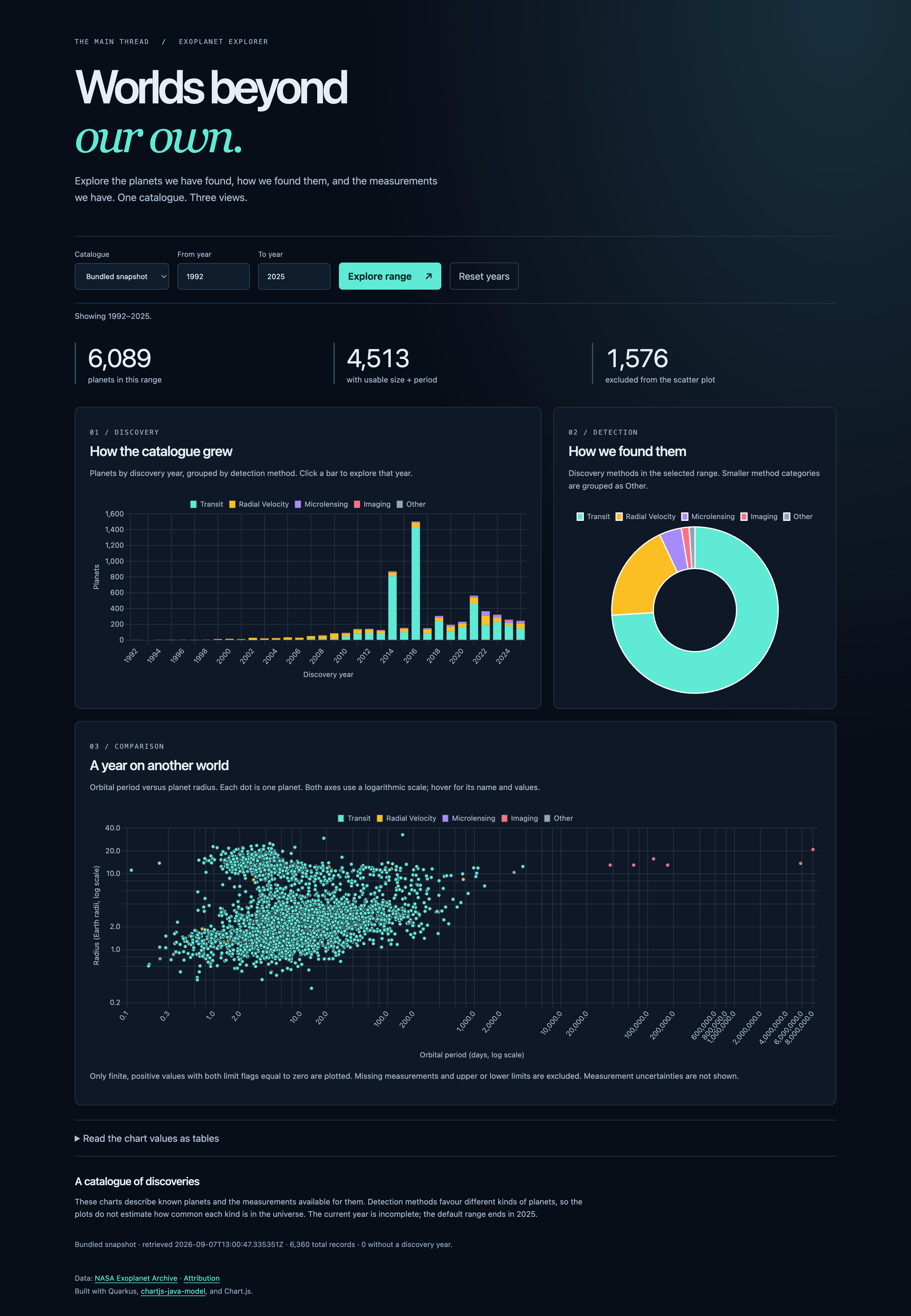
Click the 2016 bar. The controls should change to 2016–2016, the selected count should become 1,504, and the scatter should include 1,427 planets. The remaining 77 still contribute to the discovery charts. Select Reset years to restore 1992–2025; that button changes the years and keeps the currently selected source.
Use the form to try 1993–1993 with the supplied snapshot. There are no discoveries in that selection. Then try 1992–1992: there are two discoveries, but neither has the measurements required for the scatter plot. These small ranges make the empty-series behaviour easier to inspect than the full catalogue does.
Expand Read the chart values as tables to inspect the exact chart values. You can compare a method’s total with its yearly counts, or find a scatter point by planet name. Narrowing the browser window should rearrange the panels into one column without forcing the entire page to scroll horizontally.
Select NASA archive · live, then Explore range. The first request for that source calls NASA, and further range changes reuse the cached catalogue. The source line displays its retrieval time. You can exercise the same path directly:
curl -fsS 'http://localhost:8080/api/dashboard?source=live&from=2016&to=2016'Live mode can return different counts because the archive can change. If NASA is unavailable, the application returns HTTP 503 and displays the error. Choose the bundled snapshot explicitly to continue. We will test this failure path with a local fixture instead of depending on the real archive to fail.
Check invalid input directly as well:
curl -i 'http://localhost:8080/api/dashboard?from=2025&to=2000'Expect HTTP 400 and a JSON error explaining that the years must be ordered and within the supported bounds. HTML input constraints help users fill out the form, but this server-side check is what protects the endpoint when a caller bypasses the page.
Test the rules independently of NASA
The charts can render and still be wrong. We need to verify that a missing radius does not remove a discovery, an empty year keeps its place, and the response contains chart objects that the browser can use. The synthetic rows from our worked example give us stable expected results without tying the tests to today’s catalogue count.
The CLI-generated POM includes Quarkus JUnit and REST Assured as test dependencies. Create the following six files in src/test/java/com/themainthread/exoplanets. Together they cover the transformation, HTTP response, live-client integration, cache reuse, failure handling, and packaged resources.
Verify the transformation with a small fixture
Create ChartServiceTest.java:
package com.themainthread.exoplanets;

import static org.junit.jupiter.api.Assertions.assertEquals;
import static org.junit.jupiter.api.Assertions.assertFalse;
import static org.junit.jupiter.api.Assertions.assertTrue;

import java.util.List;

import org.junit.jupiter.api.Test;

import com.fasterxml.jackson.databind.ObjectMapper;

class ChartServiceTest {
    private final ChartService charts = new ChartService(new ObjectMapper());

    @Test
    void keepsCountsWhenMeasurementsAreMissingAndFillsYearGaps() {
        var catalogue = new Catalogue("fixture", "fixture", List.of(
                planet("A", "Transit", 2000, 4.0, 0, 2.0, 0),
                planet("B", "Radial Velocity", 2002, 40.0, 0, null, null),
                planet("C", "Imaging", 2002, 400.0, 1, 12.0, 0),
                planet("D", "New technique", 2002, 20.0, 0, 1.5, 0),
                planet("E", "Transit", null, 8.0, 0, 3.0, 0),
                planet("F", "Transit", 2020, 8.0, 0, 3.0, 0)));
        var dashboard = charts.build(catalogue, "snapshot", 2000, 2002);

        assertEquals(4, dashboard.selected());
        assertEquals(2, dashboard.plotted());
        assertEquals(2, dashboard.excludedFromScatter());
        assertEquals(1, dashboard.unknownYear());
        assertEquals("2001", dashboard.discoveries().at("/data/labels/1").asText());
        assertEquals(0, dashboard.discoveries().at("/data/datasets/0/data/1").asInt());
        assertEquals(1, dashboard.methods().at("/data/datasets/0/data/4").asInt());
        assertEquals("A", dashboard.sizes().at("/data/datasets/0/data/0/name").asText());
        assertEquals(4.0, dashboard.sizes().at("/data/datasets/0/data/0/x").asDouble());
        assertEquals("logarithmic", dashboard.sizes().at("/options/scales/x/type").asText());
        assertTrue(dashboard.discoveries().at("/options/scales/y/stacked").asBoolean());
        assertTrue(dashboard.sizes().at("/data/datasets/1/data").isArray());
        assertEquals(0, dashboard.sizes().at("/data/datasets/1/data").size());
    }

    @Test
    void rejectsNonPositiveNonFiniteAndBoundedValuesForLogScales() {
        for (Double value : new Double[] { null, 0.0, -1.0, Double.NaN, Double.POSITIVE_INFINITY }) {
            assertFalse(planet("A", "Transit", 2000, value, 0, 2.0, 0).hasMeasuredSizeAndPeriod());
            assertFalse(planet("A", "Transit", 2000, 2.0, 0, value, 0).hasMeasuredSizeAndPeriod());
        }
        for (Integer limit : new Integer[] { null, -1, 1 }) {
            assertFalse(planet("A", "Transit", 2000, 2.0, limit, 2.0, 0).hasMeasuredSizeAndPeriod());
            assertFalse(planet("A", "Transit", 2000, 2.0, 0, 2.0, limit).hasMeasuredSizeAndPeriod());
        }
    }

    @Test
    void emitsUsableEmptyChartConfigurations() {
        var dashboard = charts.build(new Catalogue("fixture", "fixture", List.of()), "snapshot", 2000, 2002);
        assertEquals(0, dashboard.selected());
        assertEquals(0, dashboard.plotted());
        assertEquals("doughnut", dashboard.methods().get("type").asText());
        for (var dataset : dashboard.sizes().at("/data/datasets")) {
            assertTrue(dataset.get("data").isArray());
            assertTrue(dataset.get("data").isEmpty());
        }
        assertEquals(3, dashboard.discoveries().at("/data/labels").size());
    }

    @Test
    void countsAnAbsentMethodAsOther() {
        var catalogue = new Catalogue("fixture", "fixture",
                List.of(planet("Unnamed method b", null, 2000, 4.0, 0, 2.0, 0)));
        var dashboard = charts.build(catalogue, "snapshot", 2000, 2000);
        assertEquals(1, dashboard.methods().at("/data/datasets/0/data/4").asInt());
        assertEquals(1, dashboard.plotted());
    }

    private static Planet planet(String name, String method, Integer year, Double period, Integer periodLimit,
            Double radius, Integer radiusLimit) {
        return new Planet(name, method, year, period, periodLimit, radius, radiusLimit);
    }
}
This is an ordinary JUnit test. It creates ChartService directly because the counting rules and JSON adapter do not need a running server. The first test follows our six fixture rows and checks the expected four discoveries, two plotted points, two exclusions, and one unknown year. It also checks a zero-count year, the Other group, the named point, and the emitted scale configuration.
The remaining tests exercise values that are unsuitable for logarithmic axes, a completely empty input, and an absent method. These cases are small enough to understand without inspecting thousands of NASA rows. They also make a library upgrade reviewable: if serialization stops including a field the page needs, the JSON assertions identify the changed contract.
Verify the HTTP contract and local assets
Create SnapshotTest.java:
package com.themainthread.exoplanets;

import static io.restassured.RestAssured.given;
import static org.hamcrest.Matchers.anyOf;
import static org.hamcrest.Matchers.containsString;
import static org.hamcrest.Matchers.equalTo;
import static org.hamcrest.Matchers.greaterThan;
import static org.junit.jupiter.api.Assertions.assertEquals;

import java.util.List;

import org.junit.jupiter.api.Test;

import io.quarkus.test.junit.QuarkusTest;

@QuarkusTest
class SnapshotTest {
    @Test
    void servesAllChartsAsJsonObjectsWithConsistentTotals() {
        var json = given().when().get("/api/dashboard").then().statusCode(200)
                .contentType("application/json").header("Cache-Control", "no-store")
                .body("source", equalTo("snapshot"))
                .body("selected", greaterThan(0))
                .body("discoveries.type", equalTo("bar"))
                .body("methods.type", equalTo("doughnut"))
                .body("sizes.type", equalTo("scatter"))
                .extract().jsonPath();
        List<Integer> totals = json.getList("methods.data.datasets[0].data", Integer.class);
        assertEquals(json.getInt("selected"), totals.stream().mapToInt(Integer::intValue).sum());
        assertEquals(json.getInt("selected"), json.getInt("plotted") + json.getInt("excludedFromScatter"));
    }

    @Test
    void rejectsInvalidRangesAndSources() {
        for (String query : List.of("from=2020&to=2000", "from=abc", "source=unknown", "from=1900", "to=9999")) {
            given().when().get("/api/dashboard?" + query).then().statusCode(400)
                    .body("error", anyOf(containsString("Use"), containsString("Years")));
        }
    }

    @Test
    void servesBrowserAssetsLocally() {
        given().get("/").then().statusCode(200).body(containsString("Worlds beyond"));
        given().get("/app.js").then().statusCode(200).body(containsString("new Chart"));
        given().get("/vendor/chart.umd.min.js").then().statusCode(200).body(containsString("Chart.js v4.5.1"));
    }
}
@QuarkusTest starts the application for the HTTP checks. The tests verify the chart types, source, cache-control header, total relationships, input validation, and static assets. They intentionally avoid asserting the exact number of planets in the snapshot, allowing you to refresh the data without rewriting an expected catalogue total.
The JSON path discoveries.type also checks our serialization boundary. If the resource returned a quoted chart string, that path would no longer resolve as the browser expects. The packaged Java library and the HTTP mapper therefore meet in a behaviour test, rather than relying only on their Java types compiling.
Exercise the real REST client against a local server
Create ArchiveStub.java:
package com.themainthread.exoplanets;

import java.io.IOException;
import java.net.InetSocketAddress;
import java.nio.charset.StandardCharsets;
import java.util.Map;

import com.sun.net.httpserver.HttpServer;

import io.quarkus.test.common.QuarkusTestResourceLifecycleManager;

public class ArchiveStub implements QuarkusTestResourceLifecycleManager {
    private HttpServer server;

    @Override
    public Map<String, String> start() {
        try {
            server = HttpServer.create(new InetSocketAddress("127.0.0.1", 0), 0);
            server.createContext("/TAP/sync", exchange -> {
                String query = java.net.URLDecoder.decode(exchange.getRequestURI().getRawQuery(), StandardCharsets.UTF_8);
                if (!query.contains("default_flag=1") || !query.contains("format=json")) {
                    exchange.sendResponseHeaders(400, -1);
                } else {
                    byte[] body = """
                            [{"pl_name":"Fixture b","discoverymethod":"Transit","disc_year":2001,
                              "pl_orbper":3.5,"pl_orbperlim":0,"pl_rade":1.2,"pl_radelim":0}]
                            """.getBytes(StandardCharsets.UTF_8);
                    exchange.getResponseHeaders().set("Content-Type", "application/json");
                    exchange.sendResponseHeaders(200, body.length);
                    exchange.getResponseBody().write(body);
                }
                exchange.close();
            });
            server.start();
            return Map.of("quarkus.rest-client.nasa.url", "http://127.0.0.1:" + server.getAddress().getPort());
        } catch (IOException exception) {
            throw new IllegalStateException(exception);
        }
    }

    @Override
    public void stop() {
        if (server != null) {
            server.stop(0);
        }
    }
}
The test resource starts an HTTP server on an available local port and replaces the configured NASA URL for its test. Its response uses the archive’s real column names, while the data describes one synthetic planet. It also checks that the request includes the default-solution filter and asks for JSON. This lets the real Quarkus REST client perform parameter encoding and deserialization.
Create LiveCatalogueTest.java:
package com.themainthread.exoplanets;

import static io.restassured.RestAssured.given;
import static org.hamcrest.Matchers.equalTo;
import static org.junit.jupiter.api.Assertions.assertSame;

import jakarta.inject.Inject;

import org.junit.jupiter.api.Test;

import io.quarkus.test.common.QuarkusTestResource;
import io.quarkus.test.junit.QuarkusTest;

@QuarkusTest
@QuarkusTestResource(value = ArchiveStub.class, restrictToAnnotatedClass = true)
class LiveCatalogueTest {
    @Inject
    CatalogueService catalogues;

    @Test
    void callsTapAndDeserializesItsColumnNames() {
        given().queryParam("source", "live").when().get("/api/dashboard").then().statusCode(200)
                .body("selected", equalTo(1)).body("plotted", equalTo(1))
                .body("sizes.data.datasets[0].data[0].name", equalTo("Fixture b"));
    }

    @Test
    void reusesTheCachedCatalogueAcrossRequests() {
        assertSame(catalogues.load(CatalogueService.Source.live), catalogues.load(CatalogueService.Source.live));
    }
}
Restricting the resource to this test class keeps its URL override from affecting the snapshot and failure tests. The HTTP assertion verifies that Fixture b reaches the scatter response. The cache check calls the injected service twice and expects the same catalogue instance, demonstrating that this path uses the CDI cache interceptor. It does not test the passage of an hour or cache expiration.
Keep a failed live request distinguishable from a snapshot
Create ArchiveFailureTest.java:
package com.themainthread.exoplanets;

import static io.restassured.RestAssured.given;
import static org.hamcrest.Matchers.containsString;

import java.util.Map;

import org.junit.jupiter.api.Test;

import io.quarkus.test.junit.QuarkusTest;
import io.quarkus.test.junit.QuarkusTestProfile;
import io.quarkus.test.junit.TestProfile;

@QuarkusTest
@TestProfile(ArchiveFailureTest.UnavailableArchive.class)
class ArchiveFailureTest {
    public static class UnavailableArchive implements QuarkusTestProfile {
        @Override
        public Map<String, String> getConfigOverrides() {
            return Map.of("quarkus.rest-client.nasa.url", "http://127.0.0.1:1",
                    "quarkus.rest-client.nasa.connect-timeout", "1000");
        }
    }

    @Test
    void reportsLiveFailureWithoutPretendingSnapshotDataIsLive() {
        given().queryParam("source", "live").get("/api/dashboard").then().statusCode(503)
                .body("error", containsString("Catalogue unavailable"));
        given().queryParam("source", "snapshot").get("/api/dashboard").then().statusCode(200);
    }
}
The profile points the client at an intentionally unavailable local port. The test expects a live request to return 503 and then confirms that the snapshot remains usable. You will see a warning from the deliberate failed connection during the suite. That warning is expected; the assertion is whether the application reports the failure correctly.
Repeat the HTTP checks against the packaged application
Create SnapshotIT.java:
package com.themainthread.exoplanets;

import io.quarkus.test.junit.QuarkusIntegrationTest;

@QuarkusIntegrationTest
class SnapshotIT extends SnapshotTest {
}
@QuarkusIntegrationTest repeats the inherited HTTP checks against the built application. This is where we check that the snapshot and Chart.js assets survive packaging. A successful development-mode request alone would not establish that those resources are available from the built artifact.
Stop dev mode with Ctrl+C. Then run the full verification from the module directory:
./mvnw verify -DskipITs=falseThe skipITs override enables the integration tests in the generated build. Expect ten unit/application tests and three packaged-application tests, all with zero failures and errors, followed by BUILD SUCCESS. The full suite passed for this example on 7 September 2026. The automated live-client and failure tests use local endpoints and do not call NASA.
This tutorial uses the NASA Exoplanet Archive, operated by Caltech for NASA’s Exoplanet Exploration Program; its acknowledgment page explains publication attribution.
Richard’s post gave me a reason to try the library. The catalogue shows where it fits: Java can own the grouping, measurement rules, and chart configuration alongside the application logic we already test. The browser supplies rendering and interaction, with JSON connecting the two.